5.5 Reduced Row-echelon form

The preceding section shows how to reduce a matrix to row-echelon form. However, upon conversion back to linear-equation form, back substitution is still required to achieve a solution. It turns out that back substitution can be eliminated if more work is performed on the matrix. By further reducing the matrix so there is a 1 on the diagonals, and zeroes elsewhere (except for the last column), conversion to a linear system produces equations with just a variable on one side and a constant on the other – in other words, the final solution.

Let's see how the Gauss helper can be used to do this.

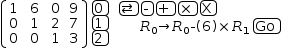
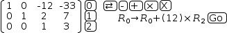
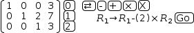
is in row-echelon form but not in reduced row-echelon form. The first step is to change the 6 in row 0 to a zero. To to this, subtract 6 times the second row from the first. The third column of row 0 is now -12, so we want to add 12 times the third row onto the first The second row starts with 0,1 so only the third column needs to be dealt with. To set it to zero, subtract twice the third row from the second. The final value of the matrix is [(1, 0, 0, 3), (0, 1, 0, 1), (0, 0, 1, 3)]. Conversion to linear-equation form gives a direct result: 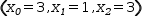(x_0=3, x_1=1, x_2=3).